In this article, we describe how we orchestrate Kafka, Dataflow and BigQuery together to ingest and transform a large stream of events. When adding scale and latency constraints, reconciling and reordering them becomes a challenge, here is how we tackle it.

 

In digital advertising, day-to-day operations generate a lot of events we need to track in order to transparently report campaign’s performances. These events come from:

• Users’ interactions with the ads, sent by the browser. These events are called tracking events and can be standard (start, complete, pause, resume, etc.) or custom events coming from interactive creatives built with Teads Studio. We receive about 10 billion tracking events a day.
• Events coming from our back-ends, regarding ad auctions’ details for the most part (real-time bidding processes). We generate more than 60 billion of these events daily, before sampling, and should double this number in 2018.

In the article we focus on tracking events as they are on the most critical path of our business.

 

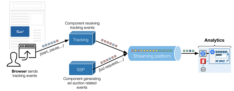
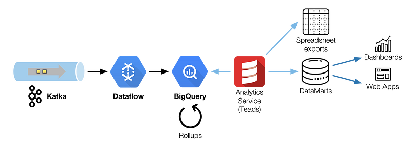
Tracking events are sent by the browser over HTTP to a dedicated component that, amongst other things, enqueues them in a Kafka topic. Analytics is one of the consumers of these events (more on that below).

We have an Analytics team whose mission is to take care of these events and is defined as follows:

We ingest the growing amount of logs,

We transform them into business-oriented data,

Which we serve efficiently and tailored for each audience.

To fulfill this mission, we build and maintain a set of processing tools and pipelines. Due to the organic growth of the company and new products requirements, we regularly challenge our architecture.

Why we moved to BigQuery

Back in 2016, our Analytics stack was based on a lambda architecture (Storm, Spark, Cassandra) and we were having several problems:

• The scale of data made it impossible to have it all in a single Cassandra table, which prevented efficient cross-querying,
• It was a complex infrastructure with code duplication for both batch and speed layers, preventing us from releasing new features efficiently,
• In the end it was difficult to scale and not cost efficient,

At that time we had several possible options. First, we could have built an enhanced lambda but it would have only postponed the problems we were facing.

We considered several promising alternatives like Druid and BigQuery. We finally chose to migrate to BigQuery because of its great set of features.

With BigQuery we are able to:

• Work with raw events,
• Use SQL as an efficient data processing language,
• Use BigQuery as the processing engine,
• Make explanatory access to date easier (compared to Spark SQL or Hive),

Thanks to a flat-rate plan, our intensive usage (query and storage-wise) is cost efficient.

However, our technical context wasn’t ideal for BigQuery. We wanted to use it to store and transform all our events coming from multiple Kafka topics. We couldn’t move our Kafka clusters away from AWS or use Pub/Sub, the managed equivalent of Kafka on GCP, since these clusters are used by some of our ad delivery components also hosted on AWS. As a result, we had to deal with the challenges of operating a multi-cloud infrastructure.

Today, BigQuery is our data warehouse system, where our tracking events are reconciled with other sources of data.

Ingestion

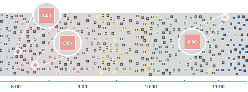
When dealing with tracking events, the first problem you face is the fact that you have to process them unordered, with unknown delays.

The difference between the time the event actually occurred (event time) and the time the event is observed by the system (processing time) ranges from the millisecond up to several hours. These large delays are not so rare and can happen when the user loses its connection or activates flight mode in between browsing sessions.

 

For further information about the challenges of streaming data processing, we recommend to have a look at Google Cloud Next ’17 talk « Moving back and forth between batch and stream processing » from Tyler Akidau (tech lead for data processing at Google) and Loïc Jaures (Teads’ co-founder and SVP Technology). The article is inspired by this talk.

The hard reality of streaming

Dataflow is a managed streaming system designed to address the challenges we face with the chaotic nature of the events. Dataflow has a unified streaming and batch programming model, streaming being the flagship feature.

We were sold on Dataflow’s promises and candidly tried streaming mode. Unfortunately, after opening it to real production traffic, we had an unpleasant surprise: BigQuery’s streaming insertion costs.

We had based our estimations on compressed data size (i.e. the actual volume of bytes that goes through the network), and not BigQuery’s raw data format size. Fortunately this is now documented for each data type so you can do the math.

Back then, we had underestimated this additional cost by a factor of 100, which almost doubled the cost of our entire ingestion pipeline (Dataflow + BigQuery). We also faced other limitations like the 100,000 events/s rate limit, which was dangerously close to what we were doing.

The good news was that there is a way to completely avoid streaming inserts limitation: batch load into BigQuery.

Ideally, we would have liked to use Dataflow in streaming mode with BigQuery in batch mode. At that time there was no BigQuery batch sink for unbounded data streams available in the Dataflow SDK.

We then considered developing our own custom sink. Unfortunately, it was impossible to add a custom sink to an unbounded data stream at the time (see Dataflow plans to add support for custom sinks that write unbounded data in a future release — it may be possible now that Beam is the official Dataflow SDK).

We had no choice but to switch our Dataflow job to batch mode. Thanks to Dataflow’s unified model it was only a matter of a few lines of code. And luckily for us, we could afford the additional data processing delay introduced by the switch to batch mode.

Moving forward, our current ingestion architecture is based on Scio, a Scala API for Dataflow open sourced by Spotify. As previously said, Dataflow natively supports Pub/Sub but Kafka integration was less mature. We had to extend Scio to enable offset checkpoint persistence and enable an efficient parallelism.

A micro batch pipeline

Our resulting architecture is a chain of 30 min Dataflow batch jobs, sequentially scheduled to read a Kafka topic and write to BigQuery using load jobs.

 

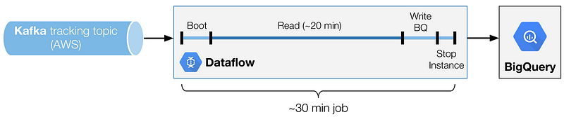
One of the key was finding the ideal batch duration. We found that there is a sweet spot to have the best trade-off between cost and reading performance (thus latency). The variable to adjust is the duration of the Kafka read phase.

To end up with the complete batch duration, you have to add the write to BigQuery phase (not proportional, but closely linked to the read duration), and a constant that is the boot and shutdown duration.

Worth noting:

• A too short reading phase will lower the ratio between reading and non-reading phases. In an ideal world, a 1:1 ratio would mean that you have to be able to read just as fast as you’re writing. In the example above, we have a 20 min read phase, for a 30 min batch (3:2 ratio). This means we have to be able to read 1.5x faster than we write. A small ratio means a need for bigger instances.
• A too long read phase will simply increase the latency between the time the event occurred and when it is available in BigQuery.

Performance tuning

Dataflow jobs are launched sequentially for simplicity reasons and easier failure management. It’s a latency trade-off we are willing to take. If a job fails we simply go back to the last commited Kafka offset.

We had to modify our Kafka clusters’ topology and increased the number of partitions to be able to unstack messages faster. Depending on the transformations you do in Dataflow, the limiting factor will most likely be the processing capacity or the network throughput. For efficient parallelism you should always try to keep a number of CPU threads that is a divisor of the number of partitions you have (corollary: it’s nice to have a number of Kafka partitions that is a highly composite number).

In the rare case of delays we are able to fine tune the job with longer read sequences. By using bigger batches, we are also able to catch up with the delay at the expense of latency.

To handle most of the situations we sized Dataflow to be able to read 3 times faster than the actual pace. A 20 min read with a single n1-highcpu-16instance can unstack 60 minutes of messages.

 

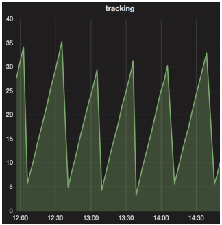
In our use case, we end up with a sawtooth latency that oscillates between 3 min (minimum duration of the Write BQ phase) and 30 min (total duration of a job).

Transformation

Raw data is inevitably bulky, we have too many events and cannot query them as is. We need to aggregate this raw data to keep a low read time and compact volumes. Here is how we do it in BigQuery:

 

Unlike traditional ETL processes where data is Transformed before it is Loaded, we choose to store it first (ELT), in a raw format.

It has two main benefits:

• It lets us have access to each and every raw event for fine analysis and debug purposes,
• It simplifies the entire chain by letting BigQuery do the transformations with a simple but powerful SQL dialect.

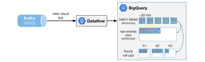
We would have liked to directly write into the raw events table that is daily partitioned. We couldn’t because a Dataflow batch has to be defined with a specific destination (table or partition) and could include data intended for different partitions. We solve this problem by loading each batch into a temporary table and then begin transforming it.

For each of these temporary batch tables, we run a set of transformations, materialized as SQL queries that output to other tables. One of these transformations simply append all the data to the big raw events table, partitioned by day.

Another of these transformations is the rollup: an aggregation of the data, given a set of dimensions. All these transformations are idempotent and can be re-run safely in case of error or need for data reprocessing.

Rollups

Querying the raw events table directly is nice for debugging and deep analysis purposes, but it’s impossible to achieve acceptable performance querying a table of this scale, not to mention the cost of such operation.

To give you an idea, this table has a retention of 4 months only, contains 1 trillion events, for a size close to 250TB.

 

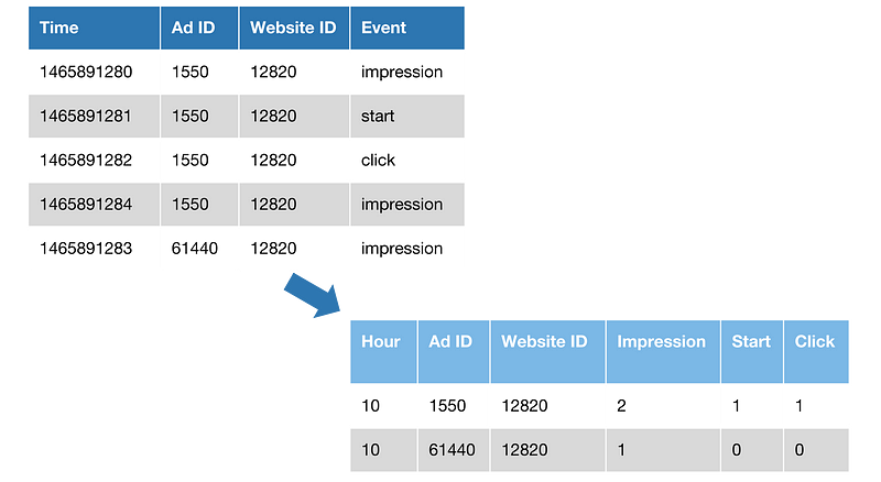
In the example above we rollup event counts for 3 dimensions: Hour, Ad ID, Website ID. Events are also pivoted and transformed to columns. The example shows a 2.5x size reduction, whereas the reality is closer to 70x.

In BigQuery’s massively parallel context, query runtime isn’t much impacted, the improvement is measured on the number of slots used.

Rollups also let us partition data into small chunks: events are grouped into small tables for a given hour (hour of the event time, not the processing time). Therefore, if you need to query the data for a given hour, you’ll query a single table (<10M rows, <10GB).

Rollups are one kind of general purpose aggregation we do to be able to query all the events more efficiently, given a large set of dimensions. There are other use cases where we want dedicated views of the data. Each of them can implement a set of specific transformations to end up with a specialized and optimized table.

Limits of a managed service

BigQuery, as powerful as it can be, has its limits:

• BigQuery doesn’t allow queries to multiple tables that have different schemas (even if the query is not using the fields that differ). We have a script to bulk update hundreds of tables when we need to add a field.
• BigQuery doesn’t support column drop. Not a big deal, but not helping to pay the technical debt.
• Querying multiple hours: BigQuery supports wildcard in table name, but performance is so bad we have to generate queries that explicitly query each table with UNION ALL.
• We always need to join these events with data hosted on other databases (e.g. to hydrate events with more information about an advertising campaign), but BigQuery does not support it (yet). We currently have to regularly copy entire tables to BigQuery to be able to join the data within a single query.

Joys of inter-cloud data transfer

With Teads’ ad delivery infrastructure in AWS and a Kafka cluster shared with many other components, we have no choice but to move quite a lot of data between both AWS and GCP Clouds, which is not easy and certainly not cheap. We located our Dataflow instances (thus the main GCP entry point) as close as possible to our AWS infrastructure, and fortunately, the existing links between AWS and GCP are good enough so we can simply use managed VPNs.

Although we encountered some instability running these VPN, we managed to sort it out using a simple script that turns it off and on again. We have never faced big enough problems to justify the cost of a dedicated link.

Once again, cost is something you have to closely watch and, where egress is concerned, difficult to assess before you see the bill. Carefully choosing how you compress data is one of the best leverage to reduce these costs.

Only halfway there

 

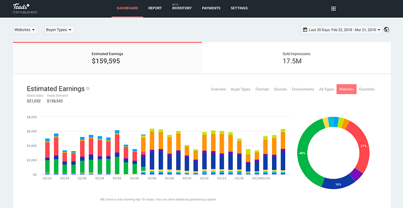
Having all these events in BigQuery is not enough. In order to bring value to the business, data has to be hydrated with different rules and metrics. Besides, BigQuery isn’t tailored for real-time use cases.

Due to concurrency limits and incompressible query latency of 3 to 5 sec (acceptable and inherent to its design), BigQuery has to be compounded with other tools to serve apps (dashboards, web UIs, etc.).

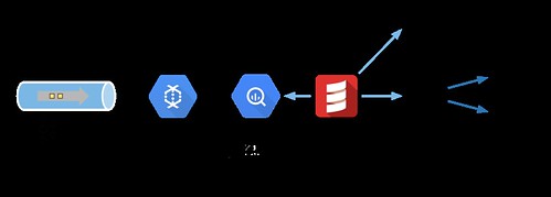
This task is performed by our Analytics service, a Scala component that taps onto BigQuery to generate on-demand reports (spreadsheets) and tailored data marts (updated daily or hourly). This specific service is required to handle the business logic. It would be too hard to maintain as SQL and generate data marts using the pipeline transformation otherwise.

We chose AWS Redshift to store and serve our data marts. Although it might not seem to be an obvious choice to serve user-facing apps, Redshift works for us because we have a limited number of concurrent users.

Also, using a key/value store would have required more development effort. By keeping an intermediate relational database, data marts consumption is made easier.

There is a lot to say on how we build, maintain and query those data marts at scale, but it will be the subject of another article.

If you like large scale event processing and Analytics related challengesgive us a shout. We are actively looking for Engineers to build tomorrow’s architecture.